8 Interpreting biplots
This section is a reminder of the possible caveats of interpreting multivariate projections (biplots) as bivariate plots (e.g., scatter plots).
The first big difference between biplots and scatter plots lies in their names. Contrary to common intuition, ‘bi’ in ‘biplot’ does not stand for two axes or dimensions but the two plots that share the same axes or dimensions. Graphically, those plots consist of points, which is analogous to a scatterplot, and arrows, which represent the covariance between variables and the dimensions of the plot. As these dimensions are given by an ordination method (e.g., PCA), they express the fact that the dataset itself has two dimensions (a matrix with rows and columns). Consequently, three-dimensional biplots are still biplots, not ‘triplots’.
There is another, more subtle, difference between biplots and scatter plots. The latter will unequivocally place points according to their values in each of the variables considered. Biplots, in turn, are projections of distributions or ‘point clouds’ that are multidimensional (i.e., multivariate data). Even in the best scenarios, biplots cannot represent such clouds in their full form. Imagine trying to draw a dice on a sheet of paper.
As an example, consider the outcome of protocol 1. In this case, robust PCA generated a good 2D projection (around 78% of variance) where CaO and MgO are the major contributors.
# Recover protocol 1 override for variable label positions
arrows_label_adj <- rbind( c(.5, -.5), c(1, .5), c(1.2, 1.2),
                           c(1.2, .4), c(.8, .5), c(0, 0),
                           c(-.2, 1), c(.5, 1.2), c(-.5, .5),
                           c(-.2, .5), c(0, .5), c(0, 0))
row.names(arrows_label_adj) <- c("Fe2O3", "Al2O3", "SiO2",
                                 "TiO2", "MgO", "Th",
                                 "Nb", "Cr", "Ce",
"Ga", "Zn", "Y")biplot_2d(prot1,
groups = factor_list$ChemGroup,
group_color = color_list$ChemGroup,
group_label_cex = 0.6,
invert_coordinates = c(TRUE, TRUE),
arrow_label_cex = 0.7,
test_text = prot1_tests$text(prot1_tests),
test_cex = 0.8,
test_fig = c(0, 0.5, 0.65, .99),
output_type = "preview")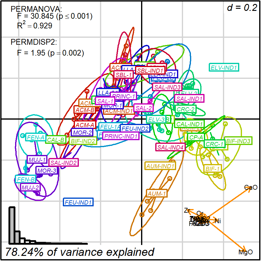
Figure 8.1: Protocol 1, representing and testing chemical reference groups
Therefore, we can safely interpret positions in terms of having more or less CaO and MgO. For instance, we can classify observations by levels of CaO content and test it against protocol 1 distance matrix and 2D projection:
# Create factor variable containing the classification (5 categories)
CaO_level <- cut(cleanAmphorae$CaO[!isShipwreck], 5)

# Select 5 colours from the 'topo.colors' palette
CaO_level_colors <- topo.colors(nlevels(CaO_level))

# Test the classification
prot1_tests_CaO <- test_groups(prot1$dist_matrix, CaO_level)
#> [1] "initiating test batch..."
#> [1] "vegan::anosim done."
#> [1] "vegan::betadisper done."
#> [1] "vegan::permutest done."
#> [1] "vegan::adonis done."
#> [1] "Test batch completed."
# This is for highlighting CaO arrow
arrow_colors <- rep("darkorange", nrow(prot1$loadings))
arrow_colors[row.names(prot1$loadings) == "CaO"] <- "red"
biplot_2d(prot1,
groups = CaO_level,
group_color = CaO_level_colors,
group_star_cex = 0,
group_label_cex = 0,
show_group_legend = TRUE,
group_legend_title = "CaO",
group_legend_title_pos = c(0.5,0.9),
group_legend_text_cex = 0.8,
group_legend_fig = c(0.7,0.99,0.68,0.95),
invert_coordinates = c(TRUE, TRUE),
arrow_label_cex = 0.8,
arrow_fig = c(.6,.95,0,.35),
arrow_label_adj_override = arrows_label_adj,
arrow_color = arrow_colors,
test_text = prot1_tests_CaO$text(prot1_tests_CaO),
test_cex = 0.8,
test_fig = c(0, 0.5, 0.65, .99),
output_type = "preview")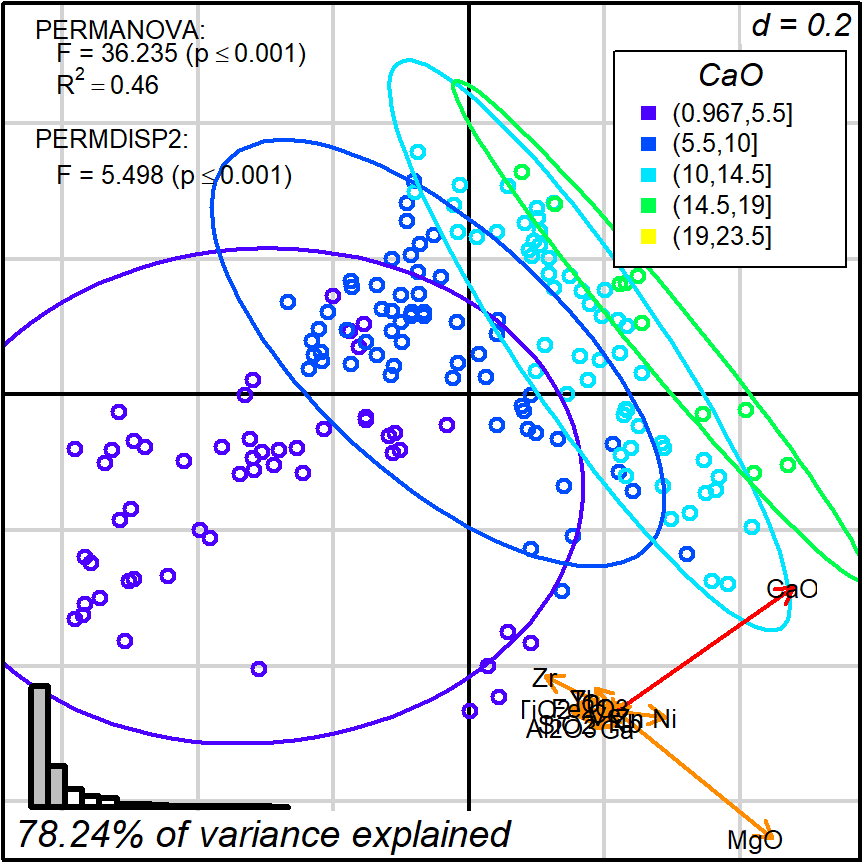
Figure 8.2: Protocol 1, grouping by level of CaO content
However, interpretation is less straightforward when more than two variables contribute significantly to the total variation. Regarding biplots, such situation implies that a smaller portion of variation is represented, and that several variables are stretch on many directions over the two principal coordinates.
For example, protocol 2 gave us a much worse 2D projection (55.7%) where fifteen variables are well represented.
# Recover protocol 2a override for variable label positions
arrows_label_adj <- rbind(c(.5,.8),c(.5,1),c(.5,1),c(.5,0),c(.5,1),
                          c(.5,0),c(0,.5))
row.names(arrows_label_adj) <- c("L48","L24","L5","L36","S7",
                                 "S8","S11")

# This will help us select different arrow colours
isDisplayed <-
  row.names(prot2a_2d$loadings) %in% row.names(
filter_arrows(prot2a_2d$loadings, min_dist = 0.5))biplot2d3d::biplot_2d(prot2a_2d,
ordination_method = "PCoA",
invert_coordinates = c (TRUE,TRUE),
xlim = c(-.26,.35),
ylim = c(-.31,.35),
point_type = "point",
groups = factor_list$FabricGroup,
group_color = color_list$FabricGroup,
group_label_cex = 0.6,
arrow_mim_dist = 0.5,
arrow_label_cex = 0.6,
arrow_fig = c(.6,.95,0,.35),
arrow_label_adj_override = arrows_label_adj,
subtitle = prot2a_2d$sub2D,
test_text = prot2a_tests$text(prot2a_tests),
test_cex = 0.8,
test_fig = c(0, 0.5, 0.65, .99),
fitAnalysis_fig = c(0,.7,.05,.5),
output_type = "preview")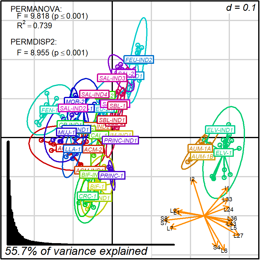
Figure 8.3: protocol 2a, representing and testing fabric groups
Like in protocol 1, we may want to interpret this projection in terms of a single variable. A obvious candidate is I2 since it is displayed long and quite isolated from other variables.
In this case, I2 (or INCLUS_ORIENT) is already a factor variable (classification) with 3 categories (plus “none” as a missing value). Note that the selected dataset will have cases in only two of those categories.
# You may want to assure that the true
# categories are corectly represented:
cleanAmphorae <- order_petro(cleanAmphorae)

levels(cleanAmphorae$INCLUS_ORIENT[!isShipwreck])
#> [1] "unparallel"        "slightly parallel" "parallel"
#> [4] "none"

# Declare this factor separately as an object for clearness
I2 <- cleanAmphorae$INCLUS_ORIENT[!isShipwreck]

# Select colours from the 'topo.colors' palette
I2_colors <- topo.colors(nlevels(I2))

# Test the classification
prot1_tests_I2 <- test_groups(prot2a_2d$dist_matrix, I2)
#> [1] "initiating test batch..."
#> [1] "vegan::anosim done."
#> [1] "vegan::betadisper done."
#> [1] "vegan::permutest done."
#> [1] "vegan::adonis done."
#> [1] "Test batch completed."
# This is for highlighting I2 arrow
arrow_colors <- rep("darkorange", nrow(prot2a_2d$loadings))
arrow_colors[row.names(prot2a_2d$loadings) == "I2"] <- "red"
# filter arrows colours, since not all variables are displayed
arrow_colors <- arrow_colors[isDisplayed]
biplot2d3d::biplot_2d(prot2a_2d,
ordination_method = "PCoA",
invert_coordinates = c (TRUE,TRUE),
xlim = c(-.26,.35),
ylim = c(-.31,.35),
groups = I2,
group_color = I2_colors,
group_star_cex = 0,
group_label_cex = 0,
show_group_legend = TRUE,
group_legend_title = "INCLUS_ORIENT",
group_legend_title_pos = c(0.5,0.9),
group_legend_text_cex = 0.8,
group_legend_fig = c(0.6,0.99,0.68,0.95),
arrow_mim_dist = .5,
arrow_label_cex = 0.8,
arrow_fig = c(.6,.95,0,.35),
arrow_label_adj_override = arrows_label_adj,
arrow_color = arrow_colors,
subtitle = prot2a_2d$sub2D,
test_text = prot1_tests_I2$text(prot1_tests_I2),
test_cex = 0.8,
test_fig = c(0, 0.5, 0.65, .99),
output_type = "preview")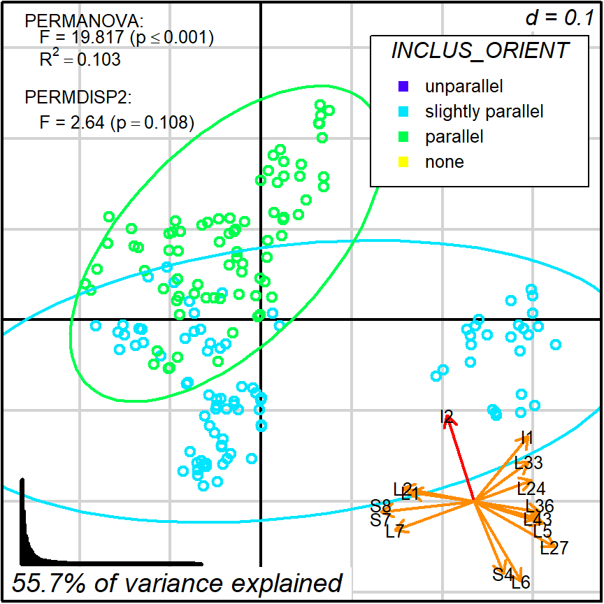
Figure 8.4: Protocol 2a, grouping by INCLUS_ORIENT
This kind of reading becomes increasingly difficult when focusing in variables that are not so well aligned, such as L33 (or COAR_R_CHERT)
# Declare this factor separately as an object for clearness
L33 <- cleanAmphorae$COAR_R_CHERT[!isShipwreck]

# Select colours from the 'topo.colors' palette
L33_colors <- topo.colors(nlevels(L33))

# Test the classification
prot1_tests_L33 <- test_groups(prot2a_2d$dist_matrix, L33)
#> [1] "initiating test batch..."
#> [1] "vegan::anosim done."
#> [1] "vegan::betadisper done."
#> [1] "vegan::permutest done."
#> [1] "vegan::adonis done."
#> [1] "Test batch completed."
# This is for highlighting L33 arrow
arrow_colors <- rep("darkorange", nrow(prot2a_2d$loadings))
arrow_colors[row.names(prot2a_2d$loadings) == "L33"] <- "red"
# filter arrows colours, since not all variables are displayed
arrow_colors <- arrow_colors[isDisplayed]
biplot2d3d::biplot_2d(prot2a_2d,
ordination_method = "PCoA",
invert_coordinates = c (TRUE,TRUE),
xlim = c(-.26,.35),
ylim = c(-.31,.35),
groups = L33,
group_color = L33_colors,
group_star_cex = 0,
group_label_cex = 0,
show_group_legend = TRUE,
group_legend_title = "COAR_R_CHERT",
group_legend_title_pos = c(0.5,0.9),
group_legend_text_cex = 0.8,
group_legend_fig = c(0.6,0.99,0.68,0.95),
arrow_mim_dist = .5,
arrow_label_cex = 0.8,
arrow_fig = c(.6,.95,0,.35),
arrow_label_adj_override = arrows_label_adj,
arrow_color = arrow_colors,
subtitle = prot2a_2d$sub2D,
test_text = prot1_tests_L33$text(prot1_tests_L33),
test_cex = 0.8,
test_fig = c(0, 0.5, 0.65, .99),
output_type = "preview")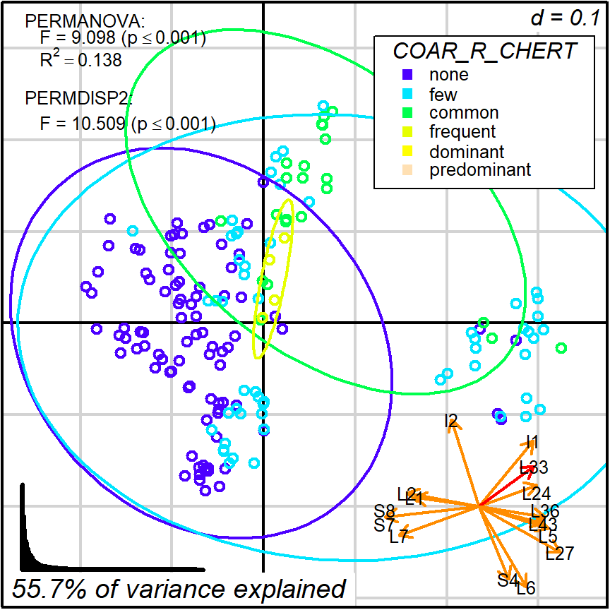
Figure 8.5: Protocol 2a, grouping by COAR_R_CHERT
Biplots and ordinal methods (PCA, PCoA, CA, etc.) are exploratory tools that play a game of compromise in order to define the best projections given the whole variance in a dataset. Do not expect them to display patterns that are clear when looking into specific variables. For that kind of analysis, you should use bivariate statistics and graphical displays, such as scatter plots or box plots.