3.4 Biplots
Ordination objects are best represented in biplots, which simultaneously display the projections of observations (points) and variables (arrows) over the same space. There are several options for creating biplots in R, starting with the readily available biplot function:
biplot(prot1)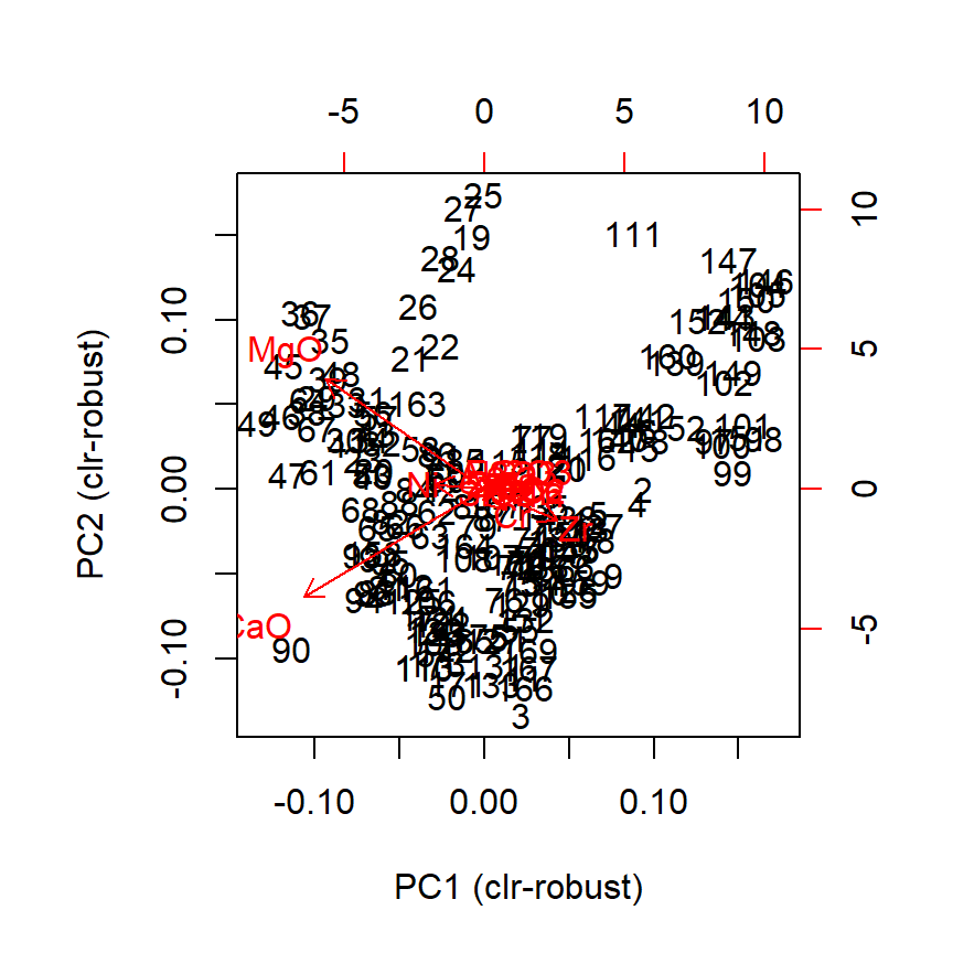
Figure 3.1: Default biplot in R
Although there are several options for customizing this default biplot function, we recommend the use of the biplot2d3d package. This package wraps a lot of possibilities in R.
library(biplot2d3d)The biplot2d3d package use functions of other packages to allow the customization of virtually all aspects of a biplot. Another important feature of this package is the creation of three-dimensional interactive biplots using the rgl package.
3.4.1 Biplot 2D
You can consult all tuning options available in the biplot_2d function by calling up the help file:
?biplot_2dThe default configuration will probably give you a much clearer picture than the biplot function, specially if your dataset contains more than 100 observations.
biplot_2d(prot1)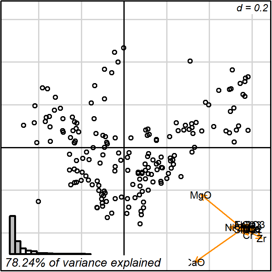
Figure 3.2: default 2D
The default setting detaches the variables projections (arrows) and places them as a miniature in the bottom-right corner. In this format they may still be interpreted, much like the North when reading a map. Remember though: the more longer arrows you see, the less each one of them is reliable when comparing point values. Here, we were ‘lucky’ for getting two nearly orthogonal variables (CaO and MgO), which means, for instance, that those observations in the bottom-left corner are surely more calcareous than those in the top-right. See the Appendix section for more details.
If detaching the arrows is not of your preference, you can disable this:
biplot_2d(prot1,
          detach_arrows = FALSE,
          output_type = "preview")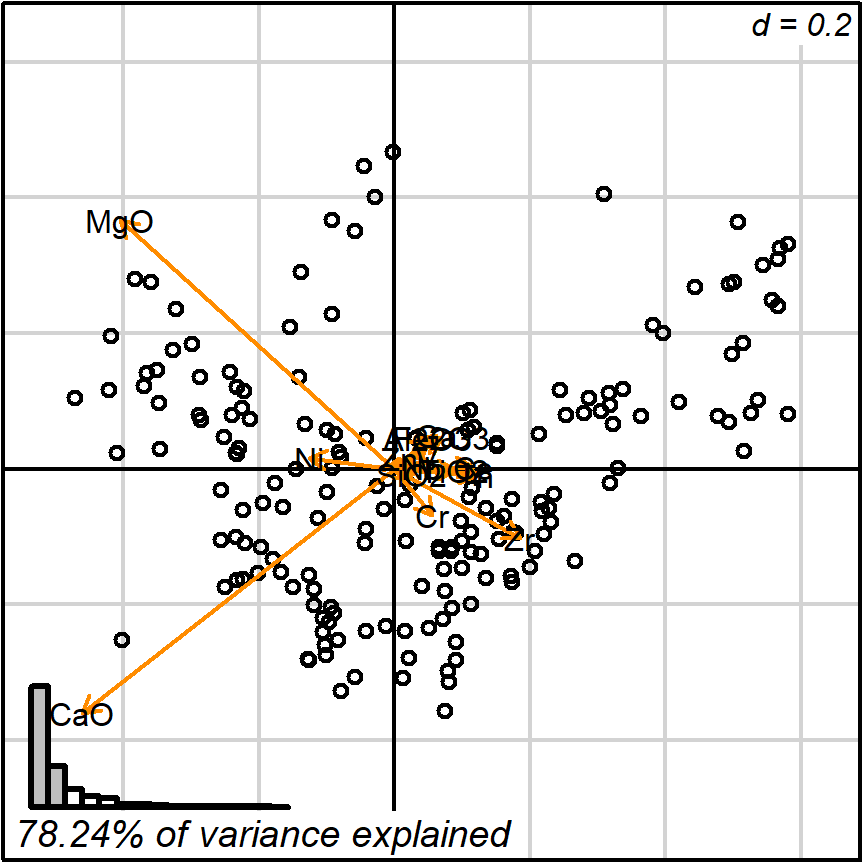
Figure 3.3: detach_arrows = FALSE
You can also visualize how the projection of points respond to a given typology (in this case, the chemical reference groups defined in previous studies).
biplot_2d(prot1,
          groups = factor_list$ChemGroup,
          output_type = "preview")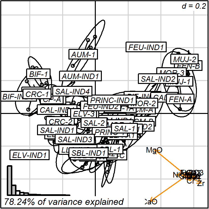
Figure 3.4: default with groups
To get a prettier plot or match your research needs, you can play with the options given by the biplot_2d.
Note that groups are by default marked using inertia ellipses. They can only be interpreted as confidence ellipses if each group can be assumed to be normally distributed in all variables considered (see more details on the scaling factor “group_ellipse_cex” in the help file). This is often not reasonable concerning groups that are either too small (< 10) or contain subgroups.
In the argument “test_text” you can introduce the “text” function of the “prot1_tests” object.
biplot_2d(prot1,
          groups = factor_list$ChemGroup,
          group_color = color_list$ChemGroup,
          group_label_cex = 0.6,
          invert_coordinates = c(TRUE, TRUE),
          arrow_label_cex = 0.7,
          test_text = prot1_tests$text(prot1_tests),
          test_cex = 0.8,
          test_fig = c(0, 0.5, 0.65, .99),
          output_type = "preview")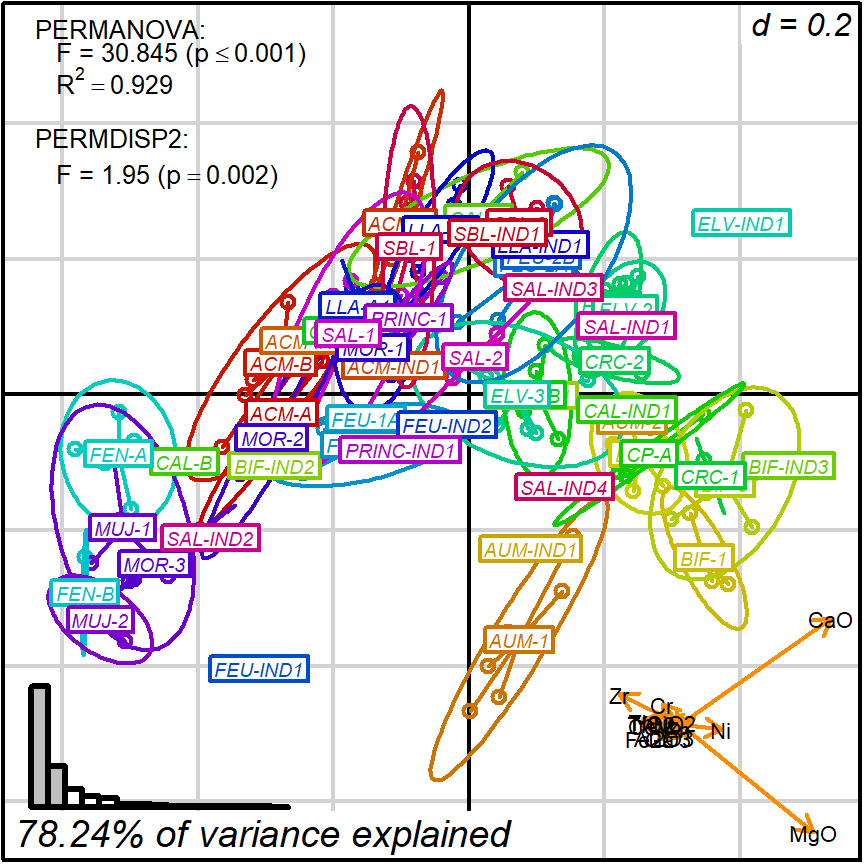
Figure 3.5: tunning appearance, groups with colors
biplot_2d(prot1,
          groups = factor_list$ChemGroup,
          group_color = color_list$ChemGroup,
          group_label_cex = 0,
          group_star_cex = 0,
          group_ellipse_cex = 0,
          point_type = "label",
          point_label = row.names(cleanAmphorae)[!isShipwreck],
          point_label_cex = 0.5,
          invert_coordinates = c(TRUE, TRUE),
          arrow_label_cex = 0.7,
          test_text = prot1_tests$text(prot1_tests),
          test_cex = 0.8,
          test_fig = c(0, 0.5, 0.65, .99),
          output_type = "preview")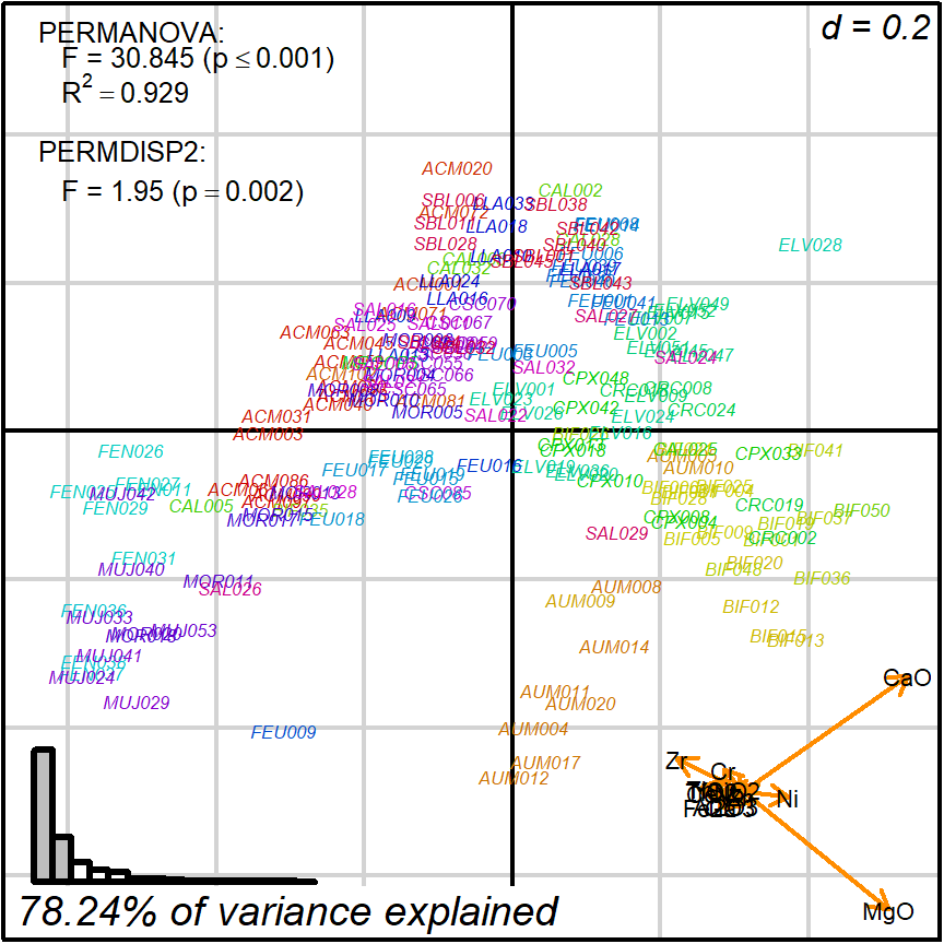
Figure 3.6: labeled points
It is also possible to save 2D biplots into various file formats (png, tiff, jpeg, eps):
# better PNG version
biplot_2d(prot1,
          ordination_method = "PCA",
          invert_coordinates = c (TRUE,TRUE),
          grid_cex = 2.5,
          ylim = c(-.1,.1),
          point_type = "point",
          groups = factor_list$ChemGroup,
          group_color = color_list$ChemGroup,
          group_label_cex = 1.5,
          arrow_label_cex = 2,
          arrow_cex = 0.2,
          arrow_lwd = 2.5,
          arrow_fig = c(.6,.95,0,.35),
          subtitle_cex = 2.5,
          test_text = prot1_tests$text(prot1_tests),
          test_fig =c(0, 0.5, 0.62, .99),
          test_cex = 2,
          fitAnalysis_fig = c(0,.7,.05,.5),
          # saving settings
          file_name = "Prot1_Biplot2D",
          directory = directories$prot1,
          width = 1000, height = 1000,
          output_type = "png")
3.4.2 Biplot 3D
Most 2D options are also available when generating 3D biplots. Consult the help file for details.
?biplot_3dbiplot_3d(prot1,
ordination_method = "PCA",
groups = factor_list$ChemGroup,
group_color = color_list$ChemGroup,
point_type = "point",
group_representation = "stars",
star_centroid_radius = 0,
star_label_cex = .8,
test_text = prot1_tests$text(prot1_tests),
test_cex = 1.25,
test_fig = c(0, 0.5, 0.65, .99))You can save an animated GIF and a PNG snapshot using the animation function.
biplot2d3d::animation(directory = directories$prot1,
                       file_name = "Prot1_Biplot3D")
You will need to install ImageMagick to be able to generate the GIF animation.
In these images, you get what you would see when running the biplot_3d function in a regular R session.
Figure 3.7: Prot1_Biplot3D.gif
NOTE: Animated GIF will not be displayed in the pdf version of this document.