3.5 Comparing CoDa transformations
There is a lot of debate on which transformation is useful–or even valid–for analyzing geochemical compositions in Archaeometry. We show here how you can compare the results of applying different transformations to the same dataset.
First, create different ordination objects for each type of CoDa transformation that you wish to compare:
prot1_std <- apply_ordination(cleanAmphorae[!isShipwreck,],
"1", # select protocol 1
coda_override = chemVars16,
coda_transformation = "std")
#> [1] "56.05% of variance explained in 2D"
#> [1] "64.91% of variance explained in 3D"
#> [1] "Protocol 1 ended."
prot1_log <- apply_ordination(cleanAmphorae[!isShipwreck,],
"1", # select protocol 1
coda_override = chemVars16,
coda_transformation = "log")
#> [1] "62.66% of variance explained in 2D"
#> [1] "72.53% of variance explained in 3D"
#> [1] "Protocol 1 ended."
prot1_ALR <- apply_ordination(cleanAmphorae[!isShipwreck,],
"1", # select protocol 1
coda_override = chemVars16,
coda_transformation = "ALR",
# this is the divisor component
coda_alr_base = "Fe2O3")
#> [1] "70.3% of variance explained in 2D"
#> [1] "81.75% of variance explained in 3D"
#> [1] "Protocol 1 ended."
prot1_CLR <- apply_ordination(cleanAmphorae[!isShipwreck,],
"1", # select protocol 1
coda_override = chemVars16,
coda_transformation = "CLR")
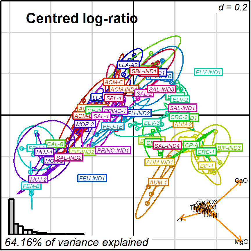
#> [1] "64.16% of variance explained in 2D"
#> [1] "75.57% of variance explained in 3D"
#> [1] "Protocol 1 ended."Then, create the respective biplots:
biplot2d3d::biplot_2d(prot1_std,
                      groups = factor_list$ChemGroup,
                      group_color = color_list$ChemGroup,
                      group_label_cex = 0.6,
                      arrow_label_cex = 0.7,
                      ylim = c(-0.9, 0.6),
                      x_title = "Scaled and Centred",
                      x_title_cex = 1.5,
                      x_title_fig = c(0.05, 0.9, 0.85, 1),
                      output_type = "preview")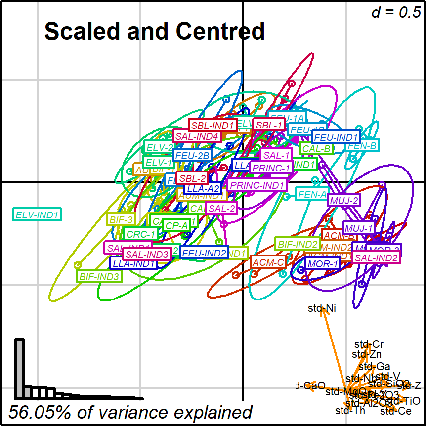
biplot2d3d::biplot_2d(prot1_log,
                      groups = factor_list$ChemGroup,
                      group_color = color_list$ChemGroup,
                      group_label_cex = 0.6,
                      arrow_label_cex = 0.7,
                      ylim = c(-0.6, 0.6),
                      x_title = "Log-scaled",
                      x_title_cex = 1.5,
                      x_title_fig = c(0.05, 0.9, 0.85, 1),
                      output_type = "preview")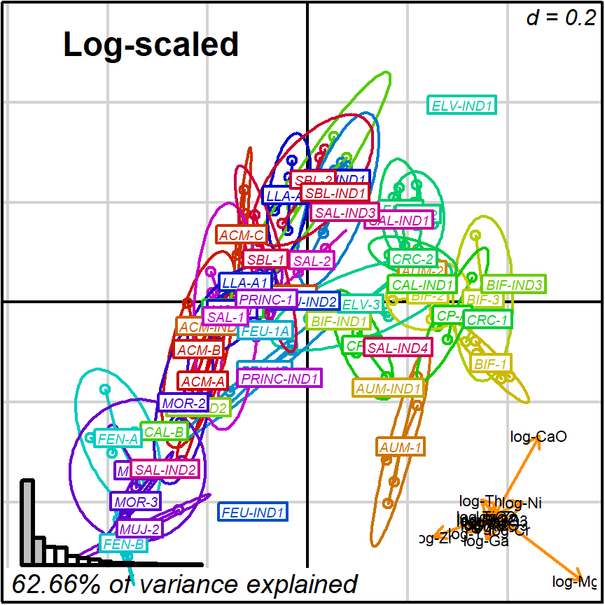
biplot2d3d::biplot_2d(prot1_ALR,
                      groups = factor_list$ChemGroup,
                      group_color = color_list$ChemGroup,
                      group_label_cex = 0.6,
                      arrow_label_cex = 0.7,
                      ylim = c(-0.6, 0.6),
                      x_title = "Additive log-ratio",
                      x_title_cex = 1.5,
                      x_title_fig = c(0.05, 0.9, 0.85, 1),
                      output_type = "preview")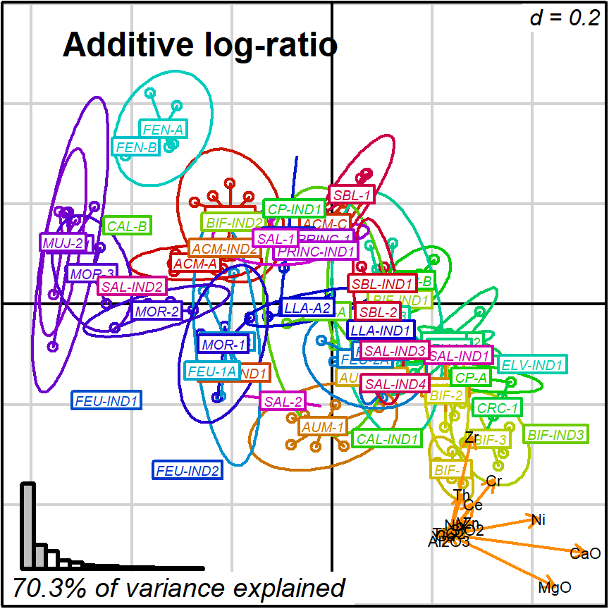
biplot2d3d::biplot_2d(prot1_CLR,
                      groups = factor_list$ChemGroup,
                      group_color = color_list$ChemGroup,
                      group_label_cex = 0.6,
                      arrow_label_cex = 0.7,
                      ylim = c(-0.5, 0.4),
                      x_title = "Centred log-ratio",
                      x_title_cex = 1.5,
                      x_title_fig = c(0.05, 0.9, 0.85, 1),
                      output_type = "preview")